Examples
This section provides practical demonstrations of how to use ChenFliessSeries.jl for computing iterated integrals, Lie derivatives, and truncated Chen–Fliess series for nonlinear control‑affine systems.
Each example illustrates a complete workflow:
Define vector fields and outputs
Compute Lie derivatives
Compute iterated integrals
Assemble the truncated Chen–Fliess series
Compare with a numerical ODE solution
Two representative systems are shown below: a 2D planar quadrotor and a nonlinear pendulum.
2D Planar Quadrotor
This example demonstrates how to compute Lie derivatives, iterated integrals, and a truncated Chen–Fliess approximation for a simplified planar quadrotor.
System dynamics
We consider the standard control–affine pendulum model:
with output
This can be written in control–affine form
where
Defining the system in Julia
 1 using Symbolics
 2 using LinearAlgebra
 3 using ChenFliessSeries
 4
 5 @variables x[1:6]
 6 x_vec = x
 7
 8 Ntrunc = 4                # truncation depth
 9 h = x[1]                  # output: horizontal position
10
11 # Physical parameters
12 gg   = 9.81
13 m    = 0.18
14 Ixx  = 0.00025
15 L    = 0.086
16
17 # Vector fields g0, g1, g2
18 g = hcat(
19     [x[4], x[5], x[6], 0, -gg, 0],
20     [0, 0, 0, 1/m*sin(x[3]), 1/m*cos(x[3]), -L/Ixx],
21     [0, 0, 0, 1/m*sin(x[3]), 1/m*cos(x[3]),  L/Ixx]
22 )
Input signal
1 dt = 0.001
2 t = 0:dt:0.1
3
4 u0 = one.(t)
5 u1 = sin.(t)
6 u2 = cos.(t)
7
8 utemp = vcat(u0', u1', u2')
Computing iterated integrals
1 E = iter_int(utemp, dt, Ntrunc)
Computing Lie derivatives
1 # Initial state
2 x_val = [0.0, 0.0, 0.1, 0.0, 0.0, 0.0]
3
4 # Build evaluator for all Lie derivatives up to Ntrunc
5 f_L = build_lie_evaluator(h, g, x_vec, Ntrunc)
6
7 # Evaluate Lie derivatives at x_val
8 L_eval = f_L(x_val)
Assembling the truncated Chen-Fliess series
1 y_cf = x_val[1] .+ vec(L_eval' * E) # output h = x1
Simulating the true 2D planar quadrotor dynamics
 1 using DifferentialEquations
 2 using Plots
 3
 4 function twodquad!(dx, x, p, t)
 5     u1 = sin(t)
 6     u2 = cos(t)
 7
 8     dx[1] = x[4]
 9     dx[2] = x[5]
10     dx[3] = x[6]
11     dx[4] = 1/m*sin(x[3])*(u1+u2)
12     dx[5] = -gg + (1/m*cos(x[3]))*(u1+u2)
13     dx[6] = (L/Ixx)*(u2-u1)
14 end
15
16 x0 = x_val
17 tspan = (0.0, 0.1)
18
19 prob = ODEProblem(twodquad!, x0, tspan)
20 sol = solve(prob, Tsit5(), saveat = t)
21
22 x1_ode = sol[1, :]
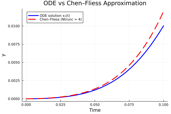
Comparison plot
 1 # Plot comparison
 2 plot(t, x1_ode,
 3     label="ODE solution x₁(t)",
 4     linewidth=3,
 5     color=:blue)
 6
 7 plot!(t, y_cf,
 8     label="Chen–Fliess (Ntrunc = 3)",
 9     linewidth=3,
10     linestyle=:dash,
11     color=:red)
12
13 xlabel!("Time")
14 ylabel!("Value")
15 title!("ODE vs Chen–Fliess Approximation")
16 plot!(grid = true)
Pendulum Example
This example illustrates how to compute a truncated Chen–Fliess series for a nonlinear pendulum with torque input and compare it with the true ODE solution.
System dynamics
We consider the standard control–affine pendulum model:
with output
This can be written in control–affine form
where
Defining the system in Julia
 1using ChenFliessSeries
 2using Symbolics
 3
 4@variables z[1:2]
 5z_vec = z
 6
 7g = hcat(
 8[z[2], -sin(z[1])],
 9[0, 1],
10)
11
12h = z[1]
Input signal
1dt = 0.001
2t = 0:dt:2.0
3
4u0 = one.(t)
5u1 = 0.5 .* sin.(2t)
6
7utemp = vcat(u0', u1')
Computing iterated integrals
1Ntrunc = 5
2E = iter_int(utemp, dt, Ntrunc)
Computing Lie derivatives
1z_val = [0.5, 0.0]
2f_L = build_lie_evaluator(h, g, z_vec, Ntrunc)
3L_eval = f_L(z_val)
Assembling the truncated Chen–Fliess series
1y_cf = z_val[1] .+ vec(L_eval' * E)
Simulating the true pendulum dynamics
 1using DifferentialEquations
 2using Plots
 3
 4function pendulum!(dz, z, p, t)
 5
 6u = 0.5*sin.(2t)
 7
 8dz[1] = z[2]
 9dz[2] = -sin(z[1]) + u
10end
11
12z0 = z_val
13prob = ODEProblem(pendulum!, z0, (0.0, 2.0))
14sol = solve(prob, Tsit5(), saveat = t)
15
16y_true = sol[1, :]
Comparison plot
1using Plots
2
3plot(t, y_cf, label="Chen–Fliess (N = $Ntrunc)", lw=2)
4plot!(t, y_true, label="True pendulum output", lw=2)
5xlabel!("t")
6ylabel!("θ(t)")
7title!("Pendulum: Chen–Fliess approximation vs ODE solution")
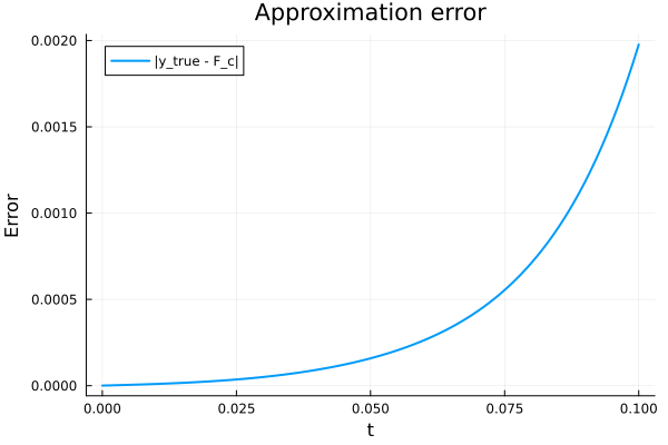
Error analysis
1err = abs.(y_true - y_cf)
2plot(t, err, label="|y_true - F_c|", lw=2)
3xlabel!("t")
4ylabel!("Error")
5title!("Approximation error")
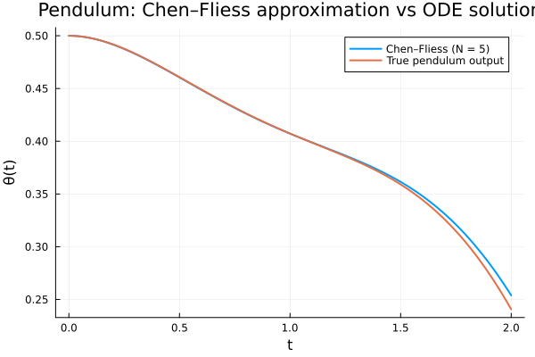
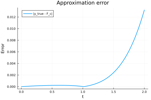
Interpretation
For small inputs and short time horizons, the truncated Chen–Fliess series provides an accurate approximation of the pendulum’s output. The error increases with:
truncation depth,
input amplitude,
and time horizon.
This example demonstrates how Chen–Fliess expansions capture nonlinear dynamics through iterated integrals and Lie derivatives, providing a powerful tool for analysis, approximation, and reachability.